The Explanation of Geographically Weighted Regression (GWR)
Geographically Weighted Regression also known as GWR is a popular method used in spatial analysis, and to model spatial relationship. One of the significance about GWR is that it provides valuable information on the nature of the processes being investigated instead of the traditional global types of regression modelling.
For instance, the Ordinary Least Squares (OLS) regression calculate a global model for the variables we are taking account for and create a single equation for the entire study area to explore their global relationship. However, the GWR provides a local model for the dependent variable at a feature point in the data set, and taking in account for each feature’s closest neighbors. In this case, it adds an extra parameter to consider for each ith-point in space to see the relationship at different location. So for example, the relationship at ith-point versus xth-point could result in different patterns.
There are reasons for performing GWR because we suspect that relationships will vary over space between our independent variable (X) and dependent variable (Y). First of all, there will inevitably be spatial variation in observed relationship because of random sampling variations. But instead, we know there are similar patterns that occur more closely to each other using the assumption of Tobler’s first law of geography therefore causes problems for statistical methods that make assumptions about the independence of residuals (a residual is the difference between an observed and a predicted value). So Moreover we are instead looking at variations that are unlikely to be due to sampling variation alone, but sources of spatial non-stationarity when simple global model cannot explain the relationship between some sets of variable. The second reason is that relationships may be intrinsically or naturally different across space. Moreover, spatial non-stationarity occur usually when there are misspecification of reality, and that relevant variables are represented by an incorrect functional form or omitted from the model.
The coefficient of determination or R square is produced from GWR represents a goodness of fit line that determines the amount of variance in the dependent variable that is correspond to the independent variable. The values range from 0 to 1 with 1 indicating the best model fit. This variable is very important to look at when determining the success of the model in explaining spatial autocorrelation, and values closer to one highlight a positive relationship and negative for negative relation, while zero shows there is no relationship.
Discussion of Geographically Weighted Regression looking at Children’s language skill in Vancouver
The objective of this case study is to perform GWR to explore the relationship between a child’s language skill (score from 1-100) and a small set of variables related to that child and to their neighbourhood. We used Exploratory regression to find the output with the highest R-squared value to determine those variables that contribute to the highest percent of variation. We added child’s social score as an additional controlled variable, and we determined that ESL, Social score, Single parent families, Recent immigrant families, and Income divided by 1000 had the strongest relationship with children’s language score. With that in mind, we performed ordinary least square analysis (OLS) and geographically weighted regression (GWR) to determine the correlation between the variables.
Grouping Analysis and GWR Results
We used grouping analysis on childcare, families of four, single parent families, recent immigrant, and income to help make sense of how locations influence those variables.
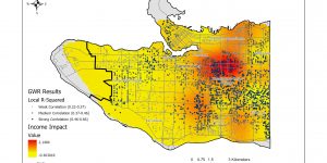
GWR on Income, Social Score, Recent Immigrant
The GWR shows that higher r squared values have higher correlation, and we are only interested in looking for areas with stronger correlation.
How GWR could be used in a variety of different context
Geographically weighted regression is very useful to help understand the relationship between variables among a spatial context. For an example, Spatial relationship exist in health geography as we examine the health factor within different regions, and highlights the importance of risks. In the paper “Area Social Deprivation and Public Health: Analyzing the Spatial Non-stationary Associations Using Geographically Weighed Regression,” is trying to find association in areas with social deprivation and see if it could provide critical implications for coping with public health risks. They look at 10 indicator to assess social deprivation, which is described from four domains: housing, education, housing and demographic structure. In addition, the performance of GWR is to help us analyze the relationship between social deprivation and incidence rate of three prevalent non-chronic disease (NCD). Although, they see that the three diseases are all positively correlated with social deprivation but the strength of the association decreases from central city to the suburb. A normal regression assumes the bases that it is the same across all space, and geography therefore play a big role here. Since there are a lot of other factors that come into play, and as well statistics sampling bias should taken into consideration. Similarly to this case study, GWR can be applied in other field of urban analysis. In a study by Chunhong Zhao, et al, GWR is used to measure the underlying factors related to surface heat island phenomenon. A urban heat island is an urban area or metropolitan area that is significantly warmer than its surrounding rural area due to human activities. Therefore, we can already assume GWR is a perfect tool to assess this phenomena because temperature is not always constant across the city. They determines that land cover composition, terrain morphology, provided different results for Austin and San Antonio. The noticeable discover Austin was also affects by spatial pattern of land use and land cover changes but its not the case for San Antonio. They need to accommodate spatial non-stationarity by allowing the model parameter to vary in space, they discovered that GWR provided spatial heterogeneity on the relationship between different land surface properties and land surface temperature. Similarly, GWR can also be applied conservational practice. In 2015, Luca Salvati conducted a study in which GWR was used to determine some latent factors and their implication for coast forest conservation in Rome, Italy. The GWR indicate the importance of urban gradient in forest dynamics because you should have a single model to represent the entire area. There are also spatial autocorrelation that we would have not been to consider, but GWR reflect scattered settlement has an influence on the disturbance to forest such as soil sealing, wildland fire, habitat fragmentation, and invasive species increase. This relationship is even stronger at areas with more mixed and heterogenous woodland structure at the urban wild interface, so therefore GWR is really crucial because we can save money and we can put our focus through sustainable land management practices on those areas. The results of GWR analysis and OLS analysis can be compared to find that differences between the two results and show indication of local variation and non-stationarity in the study. Global models like OLS are not able to detect these local variation, or accommodate for non-stationarity, their results can often be skewed or it is missing some variables. Therefore the use of GWR much more important when we consider the complexity of geography, and the science of how location affects our results.